40 format data labels excel 2016
› excel-chart-verticalExcel Chart Vertical Axis Text Labels • My Online Training Hub Apr 14, 2015 · Note how the vertical axis has 0 to 5, this is because I've used these values to map to the text axis labels as you can see in the Excel workbook if you've downloaded it. Step 2: Sneaky Bar Chart. Now comes the Sneaky Bar Chart; we know that a bar chart has text labels on the vertical axis like this: support.microsoft.com › en-us › officeChange the format of data labels in a chart To get there, after adding your data labels, select the data label to format, and then click Chart Elements > Data Labels > More Options. To go to the appropriate area, click one of the four icons ( Fill & Line , Effects , Size & Properties ( Layout & Properties in Outlook or Word), or Label Options ) shown here.
How to Print Labels from Excel - Lifewire Select Mailings > Write & Insert Fields > Update Labels . Once you have the Excel spreadsheet and the Word document set up, you can merge the information and print your labels. Click Finish & Merge in the Finish group on the Mailings tab. Click Edit Individual Documents to preview how your printed labels will appear. Select All > OK .

Format data labels excel 2016
Format Data Labels Vertically using Pareto in Excel 2016 Re: Format Data Labels Vertically using Pareto in Excel 2016. Try this: Right-click on one of the data labels > Format Data Labels > Size & Properties > Alignment > Text direction: Stacked. Register To Reply. 10-03-2017, 01:19 PM #3. 1gambit. Registered User. support.microsoft.com › en-us › officeEdit titles or data labels in a chart - support.microsoft.com To format the text in the title or data label box, do the following: Click in the title box, and then select the text that you want to format. Right-click inside the text box and then click the formatting options that you want. You can also use the formatting buttons on the Ribbon ( Home tab, Font group). EOF
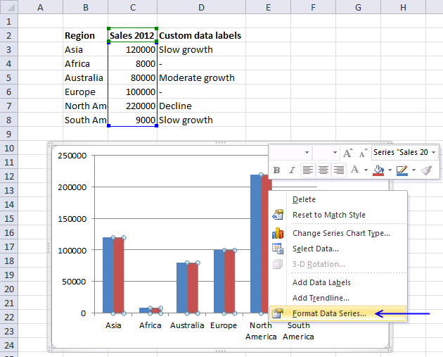
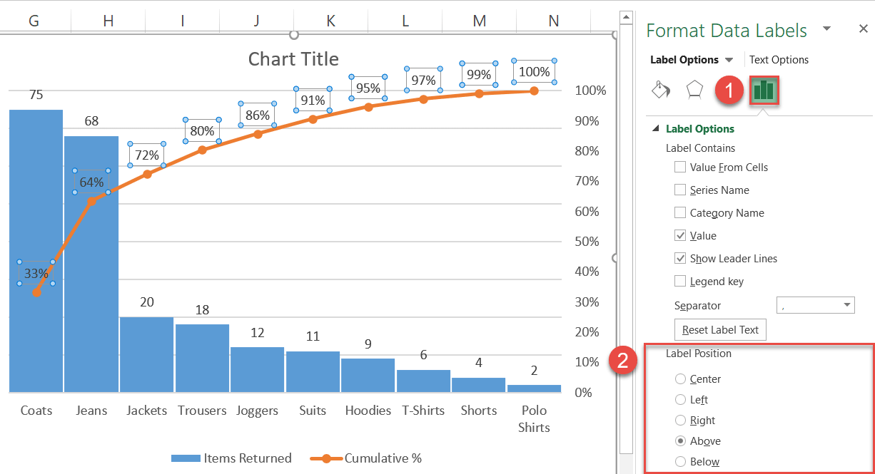
Format data labels excel 2016. How to Add Total Data Labels to the Excel Stacked Bar Chart 03.04.2013 · Step 5: Right click your new data labels and format them so that their label position is “Above”; also make the labels bold and increase the font size . Step 6: Right click the line, select “Format Data Series”; in the Line Color menu, select “No line” Step 7: Delete the “Total” data series label within the legend. Categories Excel, Visual Design Tags charts, hacks ... Change the format of data labels in a chart To get there, after adding your data labels, select the data label to format, and then click Chart Elements > Data Labels > More Options. To go to the appropriate area, click one of the four icons ( Fill & Line, Effects, Size & Properties ( Layout & Properties in Outlook or Word), or Label Options) shown here. 5 New Charts to Visually Display Data in Excel 2019 - dummies 26.08.2021 · Select the data and labels and then click Insert → Maps → Filled Map. Wait a few seconds for the map to load. Resize and format as desired. For example, you could apply one of the chart styles from the Chart Tools Design tab. To add data labels to the chart, choose Chart Tools Design → Add Chart Element → Data Labels → Show. Pouring ... Change the format of data labels in a chart To get there, after adding your data labels, select the data label to format, and then click Chart Elements > Data Labels > More Options. To go to the appropriate area, click one of the four icons ( Fill & Line, Effects, Size & Properties ( Layout & Properties in Outlook or Word), or Label Options) shown here.
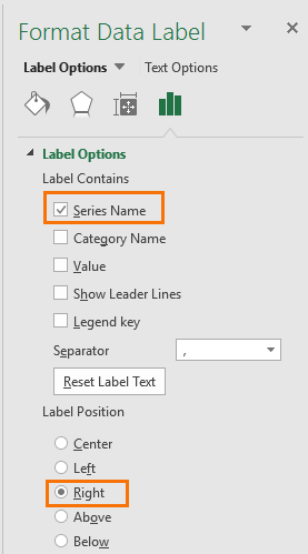
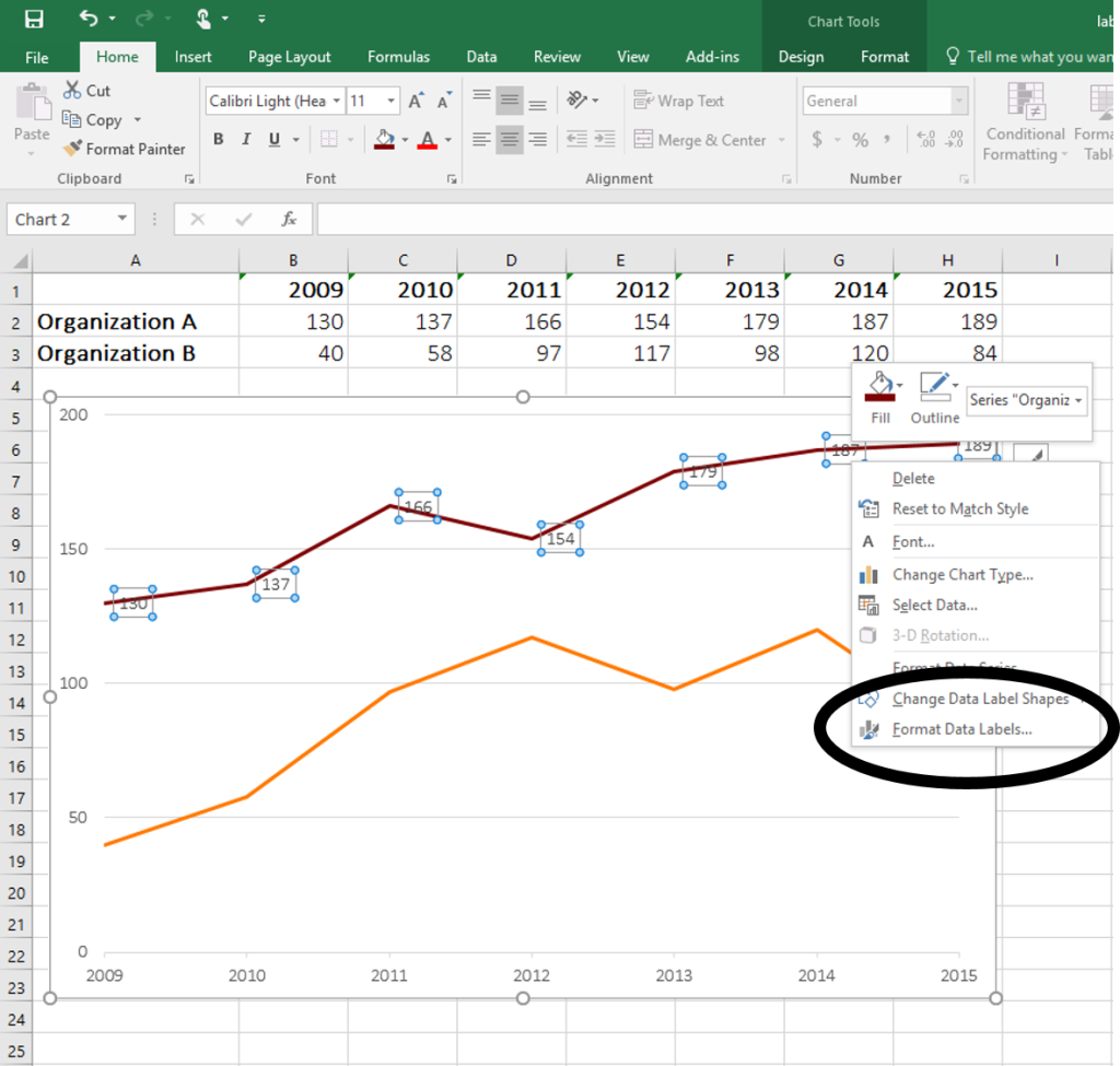
Conditional formatting for chart axes - Microsoft Excel 2016 Chart Data Format Formula Interactive chart Macro Navigation Print Protection Review Search Settings Shape Shortcuts Style Tools. Outlook All Outlook. ... To change the format of the label on the Excel 2016 chart axis, do the following: 1. Right-click in the axis and choose Format Axis ... Excel 2016 Tutorial Formatting Data Labels Microsoft Training ... - YouTube Excel 2016 Tutorial Formatting Data Labels Microsoft Training Lesson 34,315 views Jan 12, 2016 16 Dislike Share Save TeachUComp 44.9K subscribers FREE Course! Click: ... Change the format of data labels in a chart Data labels make a chart easier to understand because they show details about a data series or its individual data points. For example, in the pie chart below, without the data labels it would be difficult to tell that coffee was 38% of total sales. You can format the labels to show specific labels elements like, the percentages, series name, or category name. Excel 2016 VBA Display every nth Data Label on Chart I suggest to do following: Dim sData as Series For i = 1 to sData.Points.Count Step 4 sData.Points (i).ApplyDataLabels Next i. Note that if there is not value for the Point i in the series, the label seems not to be displayed. It took a while to find out why a label was not added to the chart.
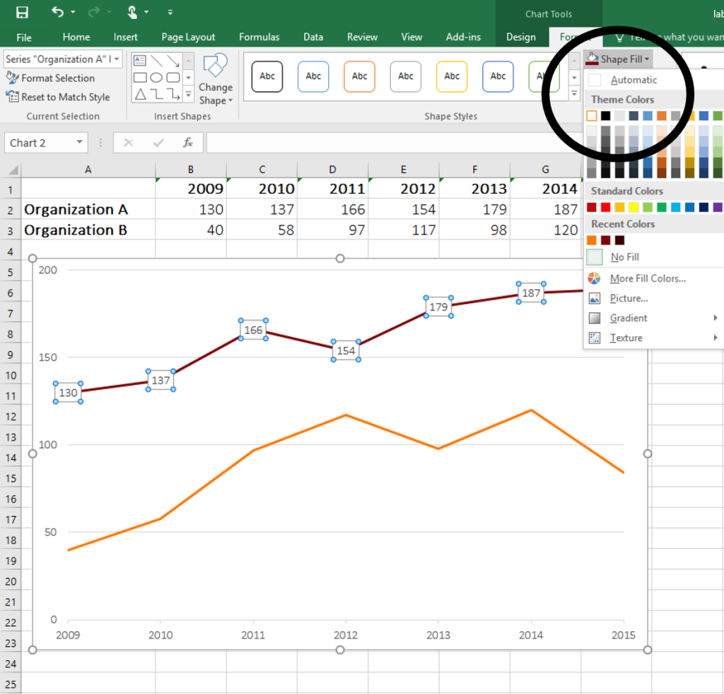
DataLabels object (Excel) | Microsoft Learn The following example sets the number format for data labels on series one on chart sheet one. With Charts(1).SeriesCollection(1) .HasDataLabels = True .DataLabels.NumberFormat = "##.##" End With Use DataLabels (index), where index is the data-label index number, to return a single DataLabel object. The following example sets the number format ... Excel charts: add title, customize chart axis, legend and data labels Click anywhere within your Excel chart, then click the Chart Elements button and check the Axis Titles box. If you want to display the title only for one axis, either horizontal or vertical, click the arrow next to Axis Titles and clear one of the boxes: Click the axis title box on the chart, and type the text. › excel › how-to-add-total-dataHow to Add Total Data Labels to the Excel Stacked Bar Chart Apr 03, 2013 · Step 4: Right click your new line chart and select “Add Data Labels” Step 5: Right click your new data labels and format them so that their label position is “Above”; also make the labels bold and increase the font size. Step 6: Right click the line, select “Format Data Series”; in the Line Color menu, select “No line” How to Format Excel Pivot Table - Contextures Excel Tips 22.06.2022 · Copy a Custom Style in Excel 2016 or Later. In Excel 2016, the custom pivot table style is not copied, if you use the above technique to copy and paste a pivot table. I found a different way to copy the custom style, and this method also works in Excel 2013. In Excel 2016, follow these steps to copy a custom style into a different workbook:
How to format Excel so that a data series is highlighted ...
blogs.library.duke.edu › data › 2012/11/12Adding Colored Regions to Excel Charts - Duke Libraries ... Nov 12, 2012 · Right-click on the individual data series to change the colors, line widths, etc. Use the formatting options or the Chart tools on the Excel ribbon to change the font of any text, adjust the grid lines, add labels and titles, etc. The data series names in the legend can be adjusted by using the “Select Data…” option and typing in custom ...
Apply Custom Data Labels to Charted Points - Peltier Tech
How to I rotate data labels on a column chart so that they are ... To change the text direction, first of all, please double click on the data label and make sure the data are selected (with a box surrounded like following image). Then on your right panel, the Format Data Labels panel should be opened. Go to Text Options > Text Box > Text direction > Rotate

How to insert data labels to a Pie chart in Excel 2013
How to create Custom Data Labels in Excel Charts - Efficiency 365 Create the chart as usual. Add default data labels. Click on each unwanted label (using slow double click) and delete it. Select each item where you want the custom label one at a time. Press F2 to move focus to the Formula editing box. Type the equal to sign. Now click on the cell which contains the appropriate label.

Change the format of data labels in a chart
File format reference for Word, Excel, and PowerPoint - Deploy … 30.09.2021 · The binary file format for Excel 2019, Excel 2016, Excel 2013, and Excel 2010 and Office Excel 2007. This is a fast load-and-save file format for users who need the fastest way possible to load a data file. Supports VBA projects, Excel 4.0 macro sheets, and all the new features that are used in Excel. But, this is not an XML file format and is therefore not optimal …

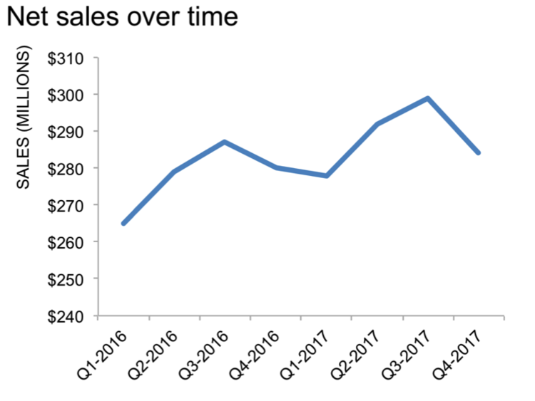
How to format axis labels as thousands/millions in Excel?
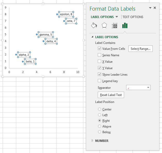
Edit titles or data labels in a chart - support.microsoft.com You can also place data labels in a standard position relative to their data markers. Depending on the chart type, you can choose from a variety of positioning options. On a chart, do one of the following: To reposition all data labels for an entire data series, click a data label once to select the data series.

How do I add Data Labels for multiple Low Points Only! : r/excel
How to rotate axis labels in chart in Excel? - ExtendOffice Rotate axis labels in Excel 2007/2010. 1. Right click at the axis you want to rotate its labels, select Format Axis from the context menu. See screenshot: 2. In the Format Axis dialog, click Alignment tab and go to the Text Layout section to select the direction you need from the list box of Text direction. See screenshot: 3. Close the dialog ...

Excel charts: add title, customize chart axis, legend and ...
› excel-pivot-table-formatHow to Format Excel Pivot Table - Contextures Excel Tips Jun 22, 2022 · Copy a Custom Style in Excel 2016 or Later. In Excel 2016, the custom pivot table style is not copied, if you use the above technique to copy and paste a pivot table. I found a different way to copy the custom style, and this method also works in Excel 2013. In Excel 2016, follow these steps to copy a custom style into a different workbook:

Custom data labels in a chart
How to Make Charts and Graphs in Excel | Smartsheet 22.01.2018 · To generate a chart or graph in Excel, you must first provide the program with the data you want to display. Follow the steps below to learn how to chart data in Excel 2016. Step 1: Enter Data into a Worksheet. Open Excel and select New Workbook. Enter the data you want to use to create a graph or chart. In this example, we’re comparing the ...

Creating Pie Chart and Adding/Formatting Data Labels (Excel)
Excel - Formatting Data Labels, Data Tables... - Microsoft Community I was trying to format data labels (adding a glow behind white text), and after it working once, when I went to change the colour, it no longer renders the glow (despite it saying it's on in the transparency &c settings on the side)! Drop shadows apply to the text boxes, not the font lettering itself, as well.
Excel 2016 Tutorial Formatting Data Labels Microsoft Training Lesson
Format Data Labels in Excel- Instructions - TeachUcomp, Inc. One way to do this is to click the "Format" tab within the "Chart Tools" contextual tab in the Ribbon. Then select the data labels to format from the "Current Selection" button group. Then click the "Format Selection" button that appears below the drop-down menu in the same area.

Improve your X Y Scatter Chart with custom data labels
How to Print Labels from Excel - Lifewire 05.04.2022 · How to Print Labels From Excel . You can print mailing labels from Excel in a matter of minutes using the mail merge feature in Word. With neat columns and rows, sorting abilities, and data entry features, Excel might be the perfect application for entering and storing information like contact lists.Once you have created a detailed list, you can use it with other …

Individually Formatted Category Axis Labels - Peltier Tech
blog.hubspot.com › marketing › how-to-build-excel-graphHow to Make a Chart or Graph in Excel [With Video Tutorial] Sep 08, 2022 · To format other parts of your chart, click on them individually to reveal a corresponding Format window. 6. Change the size of your chart's legend and axis labels. When you first make a graph in Excel, the size of your axis and legend labels might be small, depending on the graph or chart you choose (bar, pie, line, etc.)
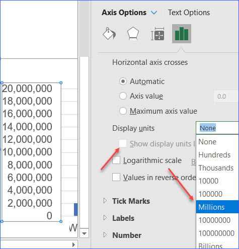
How to Format Axis Labels as Millions - ExcelNotes
Excel 2016: How to Format Data and Cells - UniversalClass.com You can apply a number format to a cell by selecting the cell (s) that you want to format, right clicking, and selecting Format Cells and select the Number tab. You can also to the Home tab, go to the Number group, then click on the arrow in the bottom right corner. You will then see the Format Cells dialogue box.
Dynamically Label Excel Chart Series Lines • My Online ...
EOF

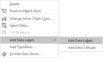
Add or remove data labels in a chart
support.microsoft.com › en-us › officeEdit titles or data labels in a chart - support.microsoft.com To format the text in the title or data label box, do the following: Click in the title box, and then select the text that you want to format. Right-click inside the text box and then click the formatting options that you want. You can also use the formatting buttons on the Ribbon ( Home tab, Font group).

Change the format of data labels in a chart
Format Data Labels Vertically using Pareto in Excel 2016 Re: Format Data Labels Vertically using Pareto in Excel 2016. Try this: Right-click on one of the data labels > Format Data Labels > Size & Properties > Alignment > Text direction: Stacked. Register To Reply. 10-03-2017, 01:19 PM #3. 1gambit. Registered User.

Change the format of data labels in a chart

Adding rich data labels to charts in Excel 2013 | Microsoft ...

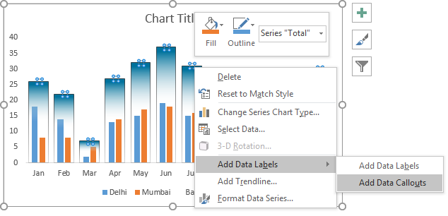
Add data labels and callouts to charts in Excel 365 ...
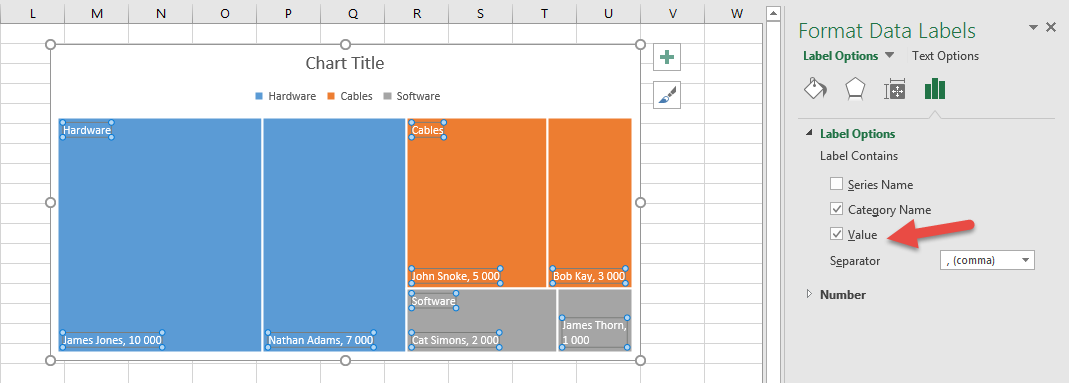
How to create a Tree Map chart in Excel 2016 | Sage Intelligence
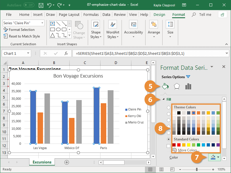
Format Excel Chart Data | CustomGuide

Format Chart Numbers as Thousands or Millions — Excel ...

How to add live total labels to graphs and charts in Excel ...
Custom data labels in a chart

Excel charts: add title, customize chart axis, legend and ...

Add or remove data labels in a chart
How to Place Labels Directly Through Your Line Graph in ...
Creating a chart with dynamic labels - Microsoft Excel 2016
Change the format of data labels in a chart
Creative Column Chart that Includes Totals in Excel

Apply Custom Data Labels to Charted Points - Peltier Tech

PCWorld
How to Place Labels Directly Through Your Line Graph in ...
How to Create a Pareto Chart in Excel – Automate Excel
Format Chart Numbers as Thousands or Millions — Excel ...
Excel axis labels - supercategory — storytelling with data

Add or remove data labels in a chart

Excel 2013 Tutorial Formatting Data Labels Microsoft Training Lesson 28.6

How to Create a Pie Chart in Excel | Smartsheet

Enable or Disable Excel Data Labels at the click of a button ...
Post a Comment for "40 format data labels excel 2016"